Discussion: We will model GDP per capita as a function of average life expectancy to determine a possible linear relationship. The hypothesis is that life expectancy will have a positive non-linear relationship with GPD (meaning that GDP will generally increase as life expectancy increases). We plan to observe a scatterplot to speculate on a possible connection and fit an appropriate regression model. Subsequently, we will test the respective models with QQ plots on the residuals and residual plots.
Simple Linear Regression for GDP and Life Expectancy
Part a. Exploratory Analysis
 |
|---|
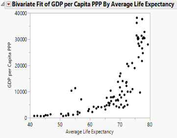
| Figure 8: GDP per capita as a function of average life expectancy. |
The scatterplot shows a strong, positive, and nonlinear relationship between GDP per capita and average life expectancy. Therefore, the GDP per capita will also increase when the average life expectancy increases. Note that there are several outliers in the plot. The outliers were not removed because they had no noticeable effect on the outcome of the model.
Part b. Model Fitting
 |
|---|
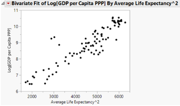
| Figure 9: log(GDP per capita) as a function of (average life expectancy)2. |
The relationship between GDP per capita and the average life expectancy was not linear. It is inappropriate to use a linear regression model to fit the data while violating the linearity assumptions. After trying different transformations on each variable, our group concluded that the variables log(GDP per capita) and (average life expectancy)2 satisfy the linear regression model’s assumptions. Additionally, the scatter plot above indicates a positive linear relationship between the two transformed variables.
 |
|---|
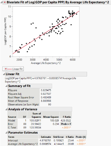
| Figure 10: JMP output of a simple linear regression model of GDP per capita as a function of average life expectancy. |
The model predicts that for every one unit increase in (average life expectancy)2, there is a corresponding 0.0008574 unit increase in the log (GDP per capita). The R2 value is 0.8295 means 82.95% of the variation in log (GDP per capita) is explained through the regression on (average life expectancy)2. Our group found that the p-value in the analysis of the variance table is less than 0.05, which indicates that the regression model statistically significantly predicts the outcome variable. Moreover, the p-value in the parameter estimates tables is also less than 0.05, which means the (average life expectancy)2 has a statistically significant effect on log (GDP per capita ppp).
Part c. Model Testing and Conclusions
 |
|---|
| Figure 11: Residual plot of studentized residual as a function of log (GDP per capita) (top). QQ plot of the studentized residuals (bottom). |
The linear regression model assumes that the error terms are independent and normally distributed with a mean 0 and a constant variance σ2. By using the residual plot and the QQ plot, our group can verify the assumptions. The points are randomly spread out in the residual plot without a discernible pattern, indicating that the variance is constant. In the QQ plot, the points fall close to the y=x line (except the outliers). Our group concludes that the residuals have an approximately normal distribution. Therefore, the simple linear regression model is appropriate for this data. Thus, as (average life expectancy)2 increases, the log(GDP per capita) increases.